
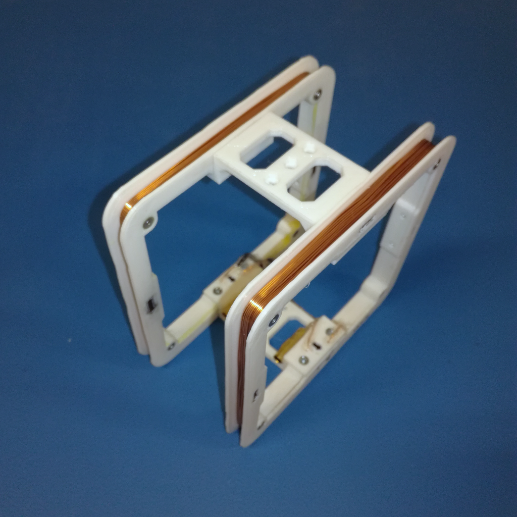
Having a way to create a uniform and controllable magnetic field in a certain volume is very useful for any workplace. This is easily achievable by building a Helmholtz Coil, two equal coils spaced apart by a certain distance. The Helmholtz Coil designed here is a small 1-Axis Helmholtz, perfect for any workbench to test magnetic sensors, acquisition system and other magnetics experiments. It is 3D printed and is designed to fit a STM32 Nucleo development board and the Mini Cube Robot.
The coils are made out of two 3D printed parts that are screwed, and possibly glued, together to reduce overhangs to a minimum and therefore simplifying 3D printing. The coils can be winded with a variety of different wire gauges (max. 1mm diameter to fit passthrough holes) and number of turns according to desired field strength and application. The wire guide rails of the coils are 7x7mm large. To get an idea and to select the best wire gauge and number of turns for the desired field strength, the Helmholtz Coil Calculator tool can be used.
The example Helmholtz Coils built here uses 30 turns of AWG24 enameled copper wire on each coil, the maximum number of turns that a spool of 10m AWG24 wire bought from AliExpress allows (it appears that the spools bought had closer to 13m of wire on it). Based on this, and using the calculator tool, the full design parameters for this Helmholtz and its expected magnetic field characteristics are as follows:
- Axis: 1-Axis
- Coil Dimension: Inner: 10x10 cm, Outer: 12x12 cm
- Coils Spacing: 5.5 cm
- Coil Turns: 30
- Field Strength: 489 $ \mathrm{\mu T} $ (4.9 Oe) with 1 A (from tool)
To drive this, and other, Helmholtz coil a simple power amplifier board is also developed. It is designed to drive 3 independent coils with bipolar current of up to 1 A from a single supply and with inexpensive power amplifiers.
Small Helmholtz Coil
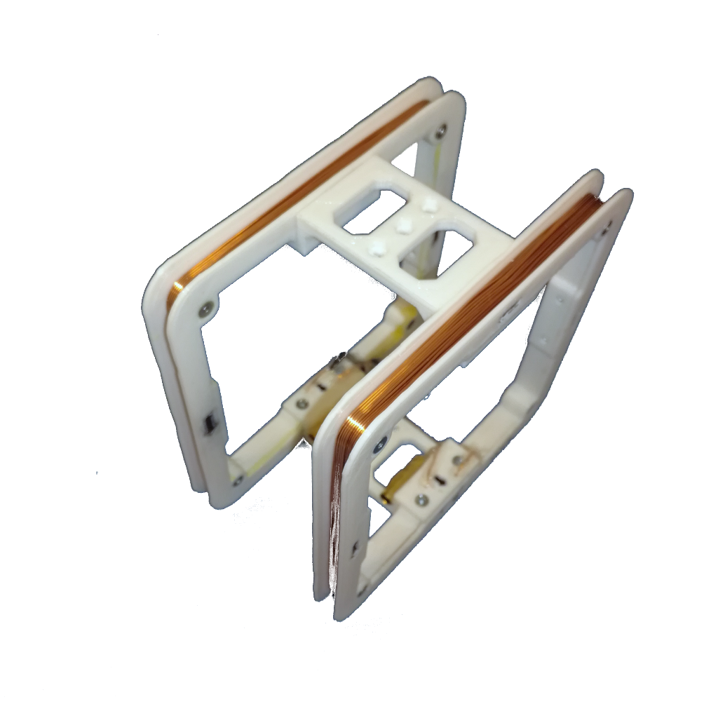
Bellow is an exploded view of the Helmholtz Coils Assembly. The parts are all 3D printed and are fit together with M2.5 countersunk screws, adding some epoxy/glue improves the adhesion between the coil base and coil covers.
Parts
Bellow is the part list required to construct this 1-Axis Helmholtz Coils. Most of the parts are 3D printed and their STL files are available for download and printing:
- Coil Base (x2): STL: Helmholtz_Small_Coil_Base.stl STEP: Helmholtz_Small_Coil_Base.step
- Coil Cover (x2): STL: Helmholtz_Small_Coil_Cover.stl STEP: Helmholtz_Small_Coil_Cover.step
- Coil Holder (x2): STL: Helmholtz_Small_Coil_Holder.stl STEP: Helmholtz_Small_Coil_Holder.step
- M2.5 Countersunk Screws: 5mm x8 and 10mm x8
- M2.5 Nuts: x22
- Enameled Copper Wire: Approx. 2*12m = 24m of AWG24 (0.5mm) Enameled Copper Wire
- Miscellaneous: 7mm wide Kapton tape
Assembly
The assembly of the Helmholtz Coils is very simple, with the step by step instructions shown bellow:
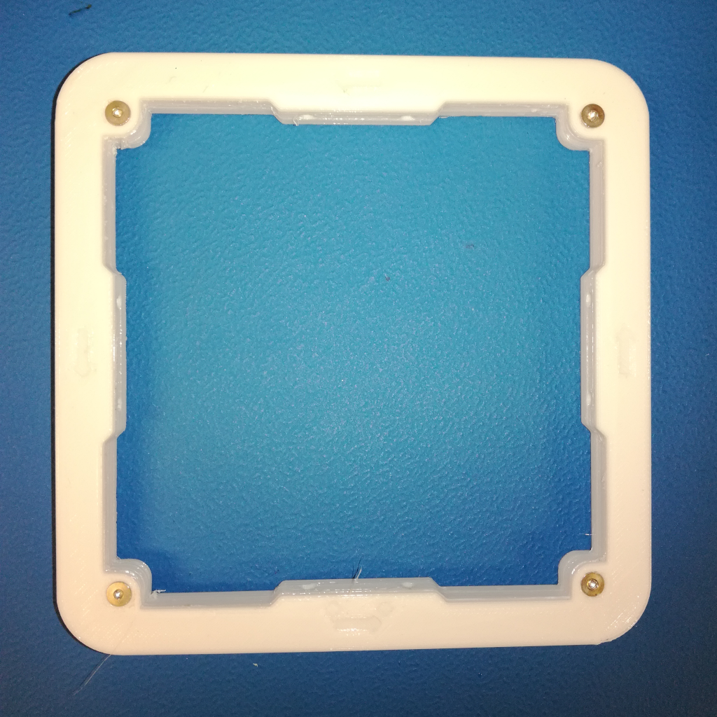
Step 1: Prepare Coil Base
First add the M2.5 nuts into the recesses in the coil base, the mounting points for the coil holders. It is possible to add holders to all 4 faces but is unnecessary, two holders on opposite faces (top and bottom) is enough. The other mounting points can be left without nuts or used to mount other things.
Because the nuts are on the inside of the coils and screwed in screws can poke out of them it is recommended to add at least one layer of Kapton, or other tape, to the inside of the coils for protection.
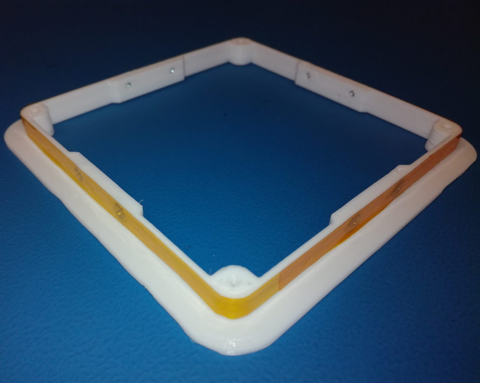
Step 2: Add Cover
Next add the cover on top of the coil base. The coil cover has arrows on each side that shows the coil winding direction and on one side two additional arrows that are used to signal the coil wire (current) input and output. Make sure to align the face with the three arrows with the coil base where the wire output holes are located.
With the cover aligned it can be screwed together with four 10mm M2.5 countersunk screws, one in each corner. Because the cover is thin and flexible it is recommended to add some glue/epoxy between the coil base and cover for better adhesion.
Step 3: Coil Winding
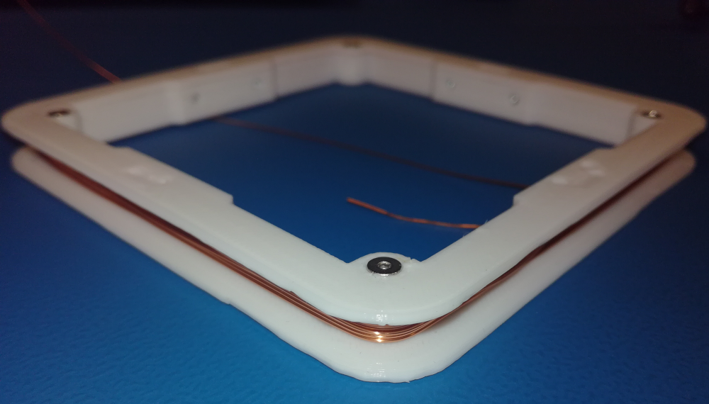
With the coil assembled, the coil windings are now added using enameled copper wire. Start by feeding a bit of wire through the coil base, through the hole more on the left, with the arrow pointing towards it on the cover. Then start winding the coils in the direction of the arrows for the desired number of turns or until running out of copper wire. The end part of the copper wire should be passed through the other hole in the coil base.
Repeat steps 1, 2 and 3 for both coils
Step 4: Screw Holders
Add the three nuts to the recesses in the middle of the coil holder, these are mounting points that can be used in the center of the Helmholtz Coil.
Take one of the coil holders and align it with the holes in the coil base, where the start/end of the coil winding are poking through. The holder has two arrows indicating the field direction when both the winding arrow and current input/output arrows are followed properly (right hand rule). Feed the start/end bits of the coil windings thorough the holder and screw it in place with two 5mm M2.5 countersunk screws to each coil.
The top coil holder is screwed in place the same way as the bottom holder, attention to that the field direction arrows are pointing in the same direction as the bottom coil holder.
Step 5: Glue Connector
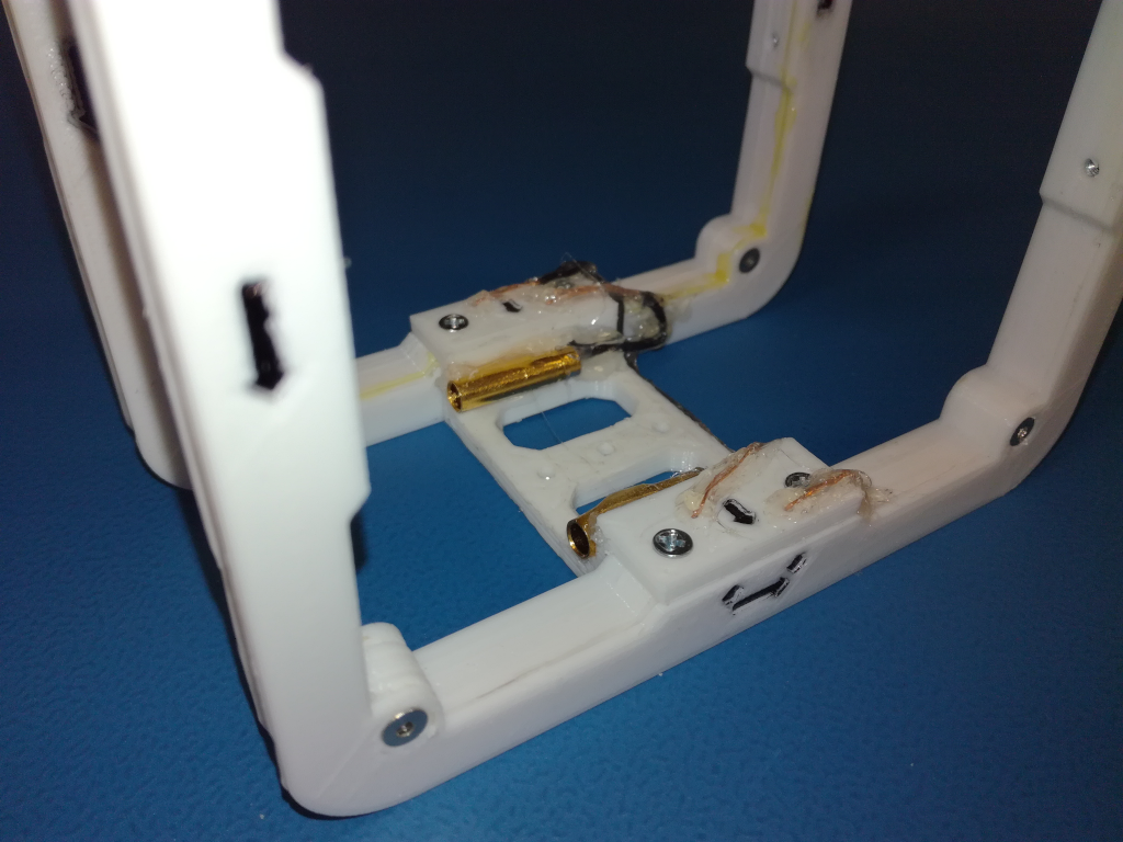
Add the three nuts to the recesses in the middle of the coil holder, these are mounting points that can be used in the center of the Helmholtz Coil.
Take one of the coil holders and align it with the holes in the coil base, where the start/end of the coil winding are poking through. The holder has two arrows indicating the field direction when both the winding arrow and current input/output arrows are followed properly (right hand rule). Feed the start/end bits of the coil windings thorough the holder and screw it in place with two 5mm M2.5 countersunk screws to each coil.
The top coil holder is screwed in place the same way as the bottom holder, attention to that the field direction arrows are pointing in the same direction as the bottom coil holder.
Step 6: Final
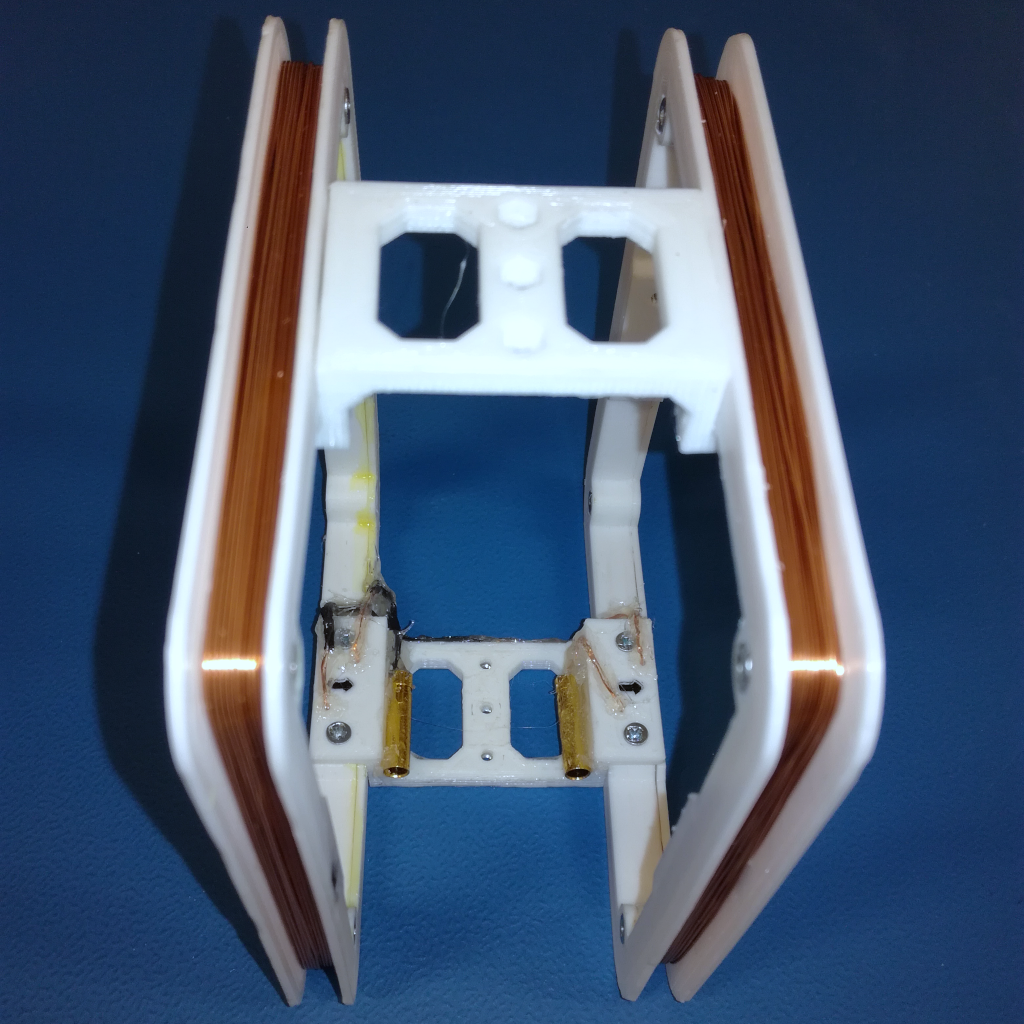
With this the Helmholtz is now fully assembled and ready to be used. By feeding a current to the banana connectors, and therefore thorough both coils, a uniform magnetic field is created in the inside of the Helmholtz Coils, proportional to the applied current.
To drive the Helmholtz Cage coils with arbitrary waveforms and with higher currents, 100’s of mA, a power amplifier is required to boost signals provided by signal generators and/or DACs. For this reason a very simple power amplifier board was designed, with the capabilities to drive up to 3 independent coils with bipolar currents of up to 1 A from a single supply and with inexpensive power amplifiers.
The first step was to select the power amplifiers to be used. The choice fell on an inexpensive high-current rail-to-rail OpAmp designed for TFT LCDs, the MAX9650 from Maxim Integrated. It has a peak output current of 1300 mA, $ \pm $ 350 mA continuos, and a supply voltage range from 6 to 20 V, according to the datasheet. The continuos current limitation is mainly dictated by the power dissipation capabilities, it has a thermal shutdown protection, and therefore a large ground plane with open pads to connect to a heatsink is important.
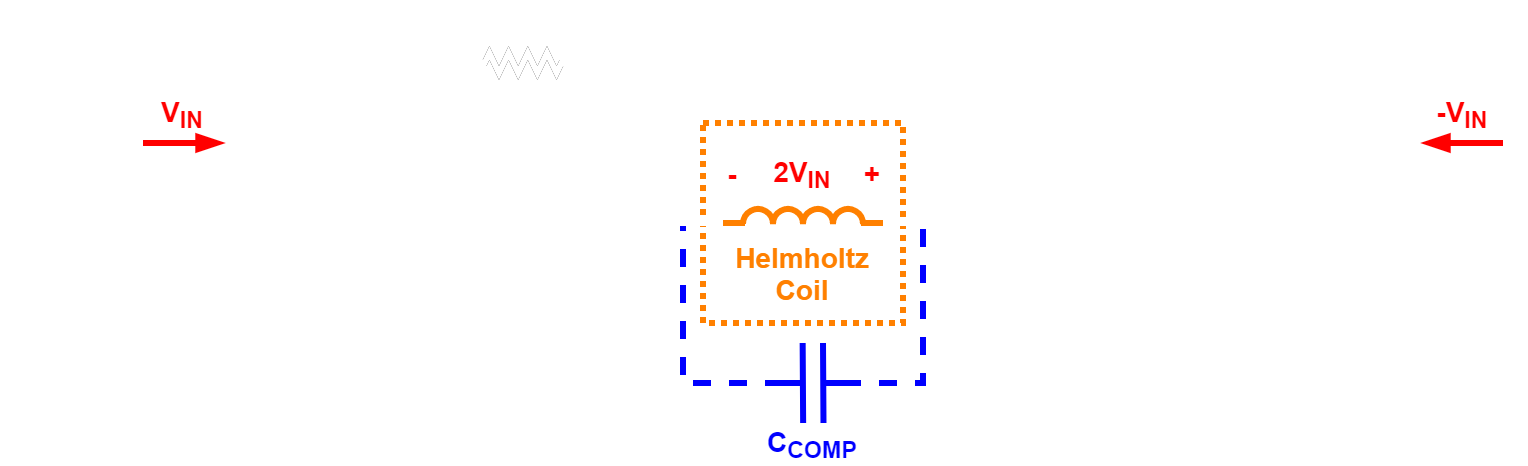
The next design challenge is to get a bipolar current drive from a single supply, no bipolar supplies with negative rails. To achieve this a bridge amplifier configuration is used (inspired from this article), where two OpAmps in a inverting configuration are used, with one OpAmps input connected to the output of the other and the load connected between their outputs. The positive input terminal of the OpAmps is used to define the bias/common voltage, creating a new mid-supply level (instead of ground) and around which the input and output will swing. The figure bellow shows a block diagram of this configuration, with $ V_{IN} $ referenced to $ V_{CM} $.
The $ V_{CM} $ is set to the mid-supply level with a buffered voltage divider. The supply can either be applied directly, through the terminal headers SUPPLY, or through a high-power buck converter on the board, which is supplied by the terminal headers VIN. The buck converter used is the LM60440, capable of delivering output currents of up to 4 A and output voltages from 3.8 V to 36 V. The output voltage of the buck converter can be set through a multi-turn potentiometer and both the output voltage and current can be monitored on a dedicated header. The output current is measured through sense resistor and an INA38. Bellow is a figure of the driver PCB.
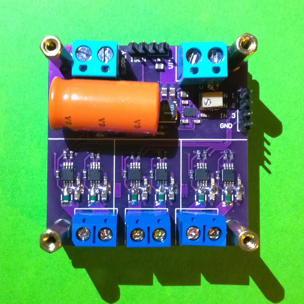
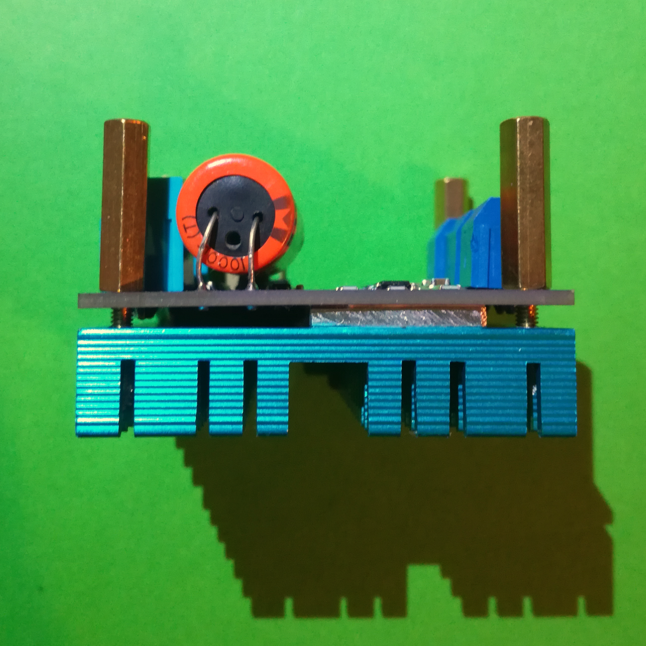
During testing some changes had to be made to get more output power/current. The first was to add a large capacitor to the output of the buck converter, above $ 1000 {\mu}F $, to stabilize the output. The next was to uncover the PCB traces leading from/to the supply and output pins of the OpAmp and adding a layer of solder on top of them to thicken the connection. The traces alone had significant voltage drops, of over 200 mV with output currents over 200 mA. Finally, to not trip the thermal shutdown protection of the OpAmps, a large 5x5cm aluminium heatsink is added to the backside of the PCB, with a aluminium piece to bridge the distance from the heatsink to the thermal pads on the backside of the PCB, as can be seen in the figure bellow.
With all these changes output currents of up to 650 mA where achieved, with a 6 V supply and the output of one channel shorted. Further tests must be performed to determine frequency response, thermal and current performance when loading all 3 channels at the same time and stability with driving coils with higher inductances.
Schematic and gerber files for this small Helmholtz Coil driver are freely available and can be downloaded from the links bellow:
Schematic: Helmholtz_Drive_Schematic_R1.pdf
Gerber: Helmholtz_Drive_Gerber_R1.zip
RL Characteristics
Each individual coil as well as the two coils in series, connected in the Helmholtz, were measured with an LCR meter. The L + R series model was used as the measurement configuration, the LCR meter measures the inductance and series DC resistance of the coil. The measurements where performed at 4 different frequencies, from 100 Hz to 100 kHz, with the results shown in the table bellow:
| Frequency | Parameter | Coil 1 | Coil 2 | Series |
|---|---|---|---|---|
| 100 Hz | LS ($ \mathrm{\mu H} $) | 244 | 244 | 544 |
| DCR ($ \Omega $) | 1.044 | 1.045 | 2.111 | |
| 1 kHz | LS ($ \mathrm{\mu H} $) | 243 | 243 | 542 |
| DCR ($ \Omega $) | 1.044 | 1.050 | 2.110 | |
| 10 kHz | LS ($ \mathrm{\mu H} $) | 242 | 242 | 538 |
| DCR ($ \Omega $) | 1.044 | 1.050 | 2.109 | |
| 100 kHz | LS ($ \mathrm{\mu H} $) | 239 | 239 | 533 |
| DCR ($ \Omega $) | 1.044 | 1.050 | 2.108 |
The first observation is that the characteristics of the coils barely change with frequency, meaning that the resonance frequency of the coil is above 100 kHz. The results are also used to confirm that each coil has the same amount of turns, easily visible in the inductance value as it increases by about 8 $ \mathrm{\mu H} $ per turn (Coil 2 initially had a larger value then Coil 1 and one turn had to be removed, one turn was “lost” when I winded that coil).
Finally, we can see that the resistance of both coils in series is almost exactly the sum of both coils resistance, results are within measurement errors. The same is not true with the inductance value. Although the sum of the inductances of each coil is close to the total inductance of the Helmholtz, the latter is higher by almost 10% (0.1). This is due to inductive coupling, mutual inductance, which happens when two coils are close enough together so that there magnetic fields interact, which is the case with a Helmholtz. The amount of inductive coupling is expressed with the coupling factor, k, and is given by the equation bellow, where M is the mutual inductance and $ L_1 $ and $ L_2 $ each coils self inductance.
$$ k = {M \over \sqrt{L_1 L_2}} $$
For the coils used here, with $ L_1 = L_2 = 244 \mathrm{\mu H} $ and $ M = 544 - 2*244 = 56 \mathrm{\mu H} $, the coupling factor is 0.23. Now, is that the expected value for the used configuration, with 10x10cm square coils spaced 5.5cm apart? According to this paper (“Scaling Law of Coupling Coefficient and Coil Size in Wireless Power Transfer Design via Magnetic Coupling” by C. Nagai et al.) yes. In the paper they present theoretical and experimental results for coupling factors vs coil dimensions and coil spacings. For a normalized coil spacing of 0.55, the value for this Helmholtz with a 10 cm “diameter” and a 5.5 cm gap, they get a theoretical coupling factor of 0.3 and an experimental factor of 0.075.
Current vs Field
The assembled Helmholtz field characteristics was obtained by feeding it with a constant current and measuring the magnetic field generated in the middle of the Helmholtz. The magnetic field was measured with an off-the-shelf cheap 3-Axis magnetometer, the QMC5883L a chinese clone of the HMC5883L, as well as with a bench gaussmeter (LakeShore Model 425). The results are shown in the figure bellow, with the results from the QMC5883L (y-axis) shown in red and from the gaussmeter in green as well as the theoretical value in dashed blue.
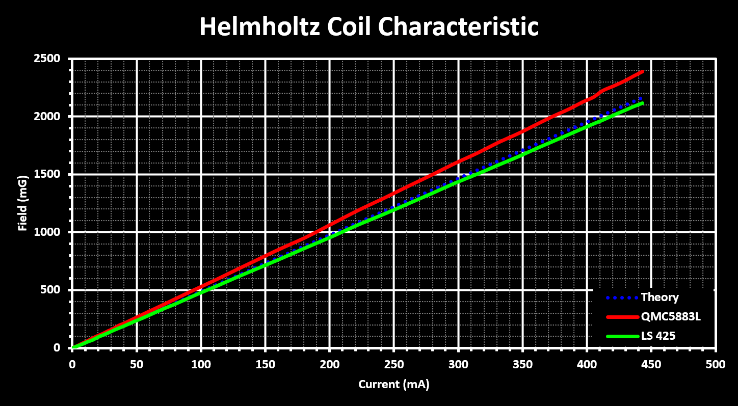
The results from the gaussmeter follow the theoretical value very closely validating the equation used, the equation from the Helmholtz Coil page. The small difference can be justified with that the real dimensions (length) of each coil is slightly larger then the value used in the calculations (10 cm), due to the windings. The difference to the cheap 3-Axis magnetometer is due to an uncalibrated sensor that is also not made to sense absolute field values with accuracy, but only for compass like applications.
The maximum field reached with the helmholtz was just above 2.1 Gauss, about 4x the earth magnetic field value (0.25-0.6 Gauss), with a drive current of 450 mA. This is far from the limit of the coils of the Helmholtz, which easily can sustain currents in the Ampere range, and it limited by the coil drive source. Larger current values will be tested at a later date.