Digital Filters

Digital Filters are one of the fundamental blocks for digital signal processing, like the analog filters are for analog signal conditioning. There are many different types of filters but the fundamental ones are the FIR and IIR filters. In general, we first simulate and tune the frequency response of the desired filter on the PC using tools like SciLab (or Matlab) or online design tools like MicroModeler.

After tuning the filter to get the required characteristics, the filter needs to be implemented in C to run on an MCU. The best and most efferent way of implementing a digital filter in an embedded system based on an ARM Cortex-M processor is using the DSP library provided by ARM, the CMSIS-DSP library. It provides functions for both FIR and IIR filters that are highly optimized. Some newer MCUs feature dedicated hardware accelerated filter calculation units that can be used to offload some of these digital filters, e.g. the FMAC on some STM32 MCUs which I explore in the DSP Accelerators page.

There is also the question of which number format to use, fixed-point or floating point. This depends mostly on the application and the chosen MCU. Fixed-point math is often preferred in embedded systems as it is faster to compute, when no floating point arithmetics unit (FPU) is present, and doesn’t require conversions as most sensors and ADCs/DACs use integers/fixed-point notations already.

Finite Input Response (FIR) Filter is a filter with a finite impulse response, it settles to zero after a finite, N + 1 samples, amount of time. It is constructed without feedback, N amounts of previous inputs are multiplied and summed up to give the filter output. These are called Taps. The simplest form of a FIR filter is the moving average, or rolling average, which is often used without even seeing it as a “real” filter. For it all coefficients are the same and equal to $ 1 \over {N_{Taps}} $. More complex and different frequency responses are accomplished by changing the values of the coefficients.

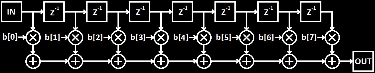
Bellow is a block diagram of a 8 Tap FIR filter, $ Z^{-1} $ is a delay of 1 sample and b[N] are the coefficients for each Tap:

A FIR filter can easily be designed with SciLab by using the ffilt(ft,n,fl,fh) function. It uses 4 parameters:

• ft: Filter type: ‘lp’ for low-pass, ‘hp’ for high-pass, ‘bp’ for band-pass, ‘sb’ for stop-band
• n: Number of Taps
• fl: First cut-off frequency
• fh: Second cut-off frequency (not used for ‘lp’ or ‘hp’).

The function then returns an array with the coefficients for the FIR filter.

To get/draw the filter response the function frmag(sys,npts) is used where the first parameter, sys, is the coefficients array and the second, npts, the number of points to calculate for the frequency response. Bellow is an example of using all these to draw the frequency response of a FIR low-pass filter with 8 Taps and a cut-off frequency of $ 0.1 * F_{S} $:

hn = ffilt('lp', 8, 0.1, 0);			//Generate FIR Filter Coefficients
[hzm, fr] = frmag(hn, 256);				//Generate Filter Response Curve
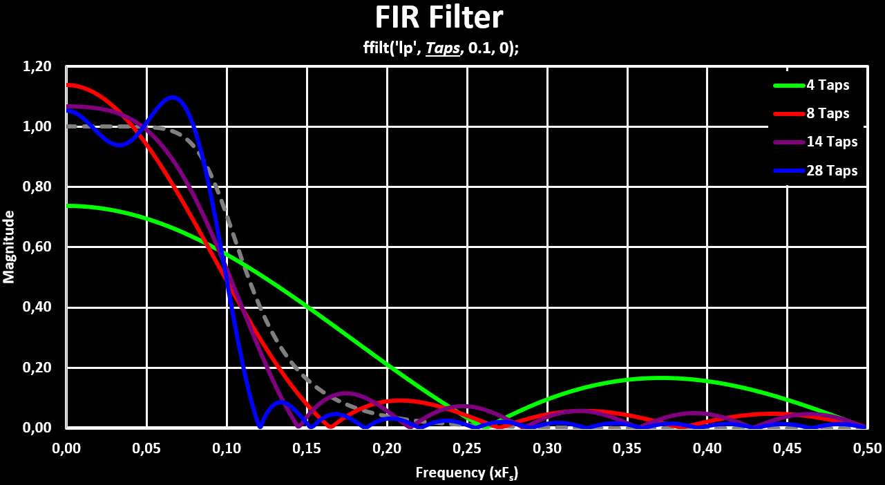
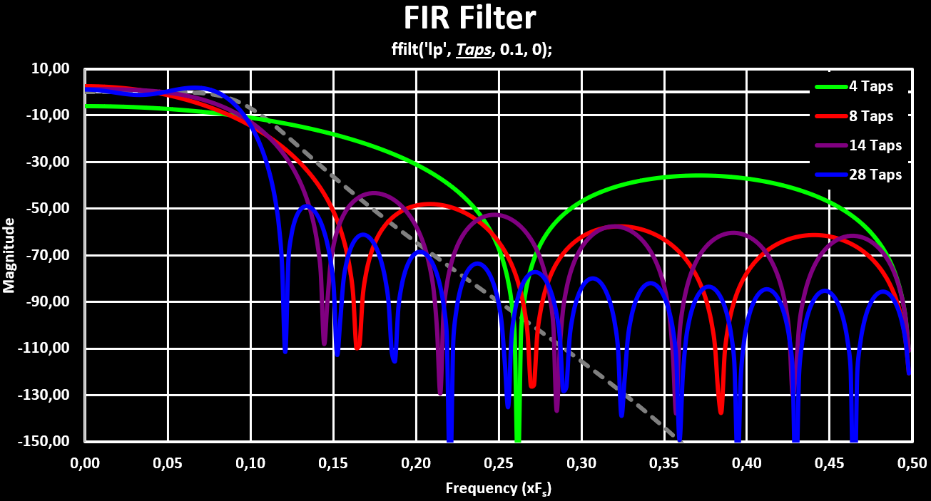
plot(fr', hzm');						//Draw Filter Response Curve

Bellow is a figure that shows the change of the frequency responses with the increase of the number of Taps. Both with linear magnitude and with logarithmic magnitude, $ 20 * log(mag) $. In grey dashed is a 4th Order IIR filter for reference:

Linear Log (dB)

Implementation on ARM MCU (CMSIS-DSP)

The CMSIS-DSP library provides functions for the implementation of the FIR filter in fixed point format, both Q15 and Q31, as well as in float format in F32. A good resource to see how to use each function can be found on this page.

The first thing to do is to initialize the filter structure by using the arm_fir_init_q15(S, numTaps, pCoeffs, pState, blockSize) or arm_fir_init_q31(S, numTaps, pCoeffs, pState, blockSize) or arm_fir_init_float(S, numTaps, pCoeffs, pState, blockSize) functions. These functions expect 5 parameters:

• S: Pointer to the filter structure (arm_fir_instance_q15, arm_fir_instance_q31, arm_fir_instance_f32)
• numTaps: Number of Taps of the FIR filter
• pCoeffs: Pointer to the filter coefficient array
• pState: Pointer to a state buffer array (used internally as the delay line under others)
• blockSize: Block size aka how many samples are processed with each filter function call, often just 1 sample at a time.

For the fixed-point version, the first thing to do is to convert the coefficients calculated by SciLab into the appropriate fixed point format. For Q15 this is done by multiplying the coefficients by $ 2^{15} $ and for Q31 by $ 2^{31} $, and then rounding them to an integer.

The coefficients have to be in reversed order and in case of the Q15 version the number of Taps has to be greater then 4 and even. If an odd number of Taps is to be used the last coefficient is set to 0. Also, the state buffer has to be of length $ nTaps + blockSize - 1 $ for both Q31 and Float version, and $ nTaps + blockSize$ for the Q15 version.

Bellow is example code used to initialize each version of the FIR filter, using the same filter coefficients calculated with the SciLab code above:

//Q15 FIR Filter
uint16_t blockLen = 1;
int16_t firStateQ15[8 + blockLen];
// 						b[tabs-1], 	b[tabs-2], ..., 			b[1], b[0]
int16_t firCoeffQ15[8] = {	2411, 4172, 5626, 6446, 6446, 5626, 4172, 2411};
arm_fir_instance_q15 armFIRInstanceQ15;
arm_fir_init_q15(&armFIRInstanceQ15, 8, firCoeffQ15, firStateQ15, blockLen);

//Q31 FIR Filter
uint16_t blockLen = 1;
int32_t firStateQ31[8 + blockLen - 1];
// 							b[tabs-1], 	b[tabs-2], ..., 										b[1], 		b[0]
int32_t firCoeffQ31[8] = {	158004550, 273426110, 368677283, 422466574, 422466574, 368677283, 273426110, 158004550 };
arm_fir_instance_q31 armFIRInstanceQ31;
arm_fir_init_q31(&armFIRInstanceQ31, 8, firCoeffQ31, firStateQ31, blockLen);

//Float FIR Filter
uint16_t blockLen = 1;
float firStateF32[8 + blockLen - 1];
// 						b[tabs-1], 	b[tabs-2], ..., 										b[1], 		b[0]
float firCoeffF32[8] = { 0.0735766, 0.127324, 0.1716787, 0.1967263, 0.1967263, 0.1716787, 0.127324, 0.0735766 };
arm_fir_instance_f32 armFIRInstanceF32;
arm_fir_init_f32(&armFIRInstanceF32, 8, firCoeffF32, firStateF32, blockLen);

After the initialization the filter is now ready to be used. To apply the filter to a new input sample the arm_fir_q15(S, pSrc, pDst, blockSize) or arm_fir_q31(S, pSrc, pDst, blockSize) or arm_fir_f32(S, pSrc, pDst, blockSize) function is called, which expects 4 parameters:

• S: Pointer to the filter structure
• pSrc: Pointer to the input samples (an array when block size > 1)
• pDst: Pointer to where write the output filtered samples (an array when block size > 1)
• blockSize: Block length, how many samples to process in one call

Bellow is example code on how to use each of these filter functions. In case of the fixed point implementations, there is a _fast version for each of them that is slightly faster but does not do any overflow protection and so the input has to be scaled to prevent overflow, by log2(number of Taps) bits. In general, the performance gain is so minimal that it is not worth the complications that can happen, as can be seen in the benchmark section.

//Q15 FIR Filter
uint16_t blockLen = 1;
int16_t inputSample;
int16_t filteredSample;
arm_fir_q15(&armFIRInstanceQ15, &inputSample, &filteredSample, blockLen);
//Slightly faster but no overflow protection
//arm_fir_fast_q15(&armFIRInstanceQ15, &inputSample, &filteredSample, blockLen);

//Q31 FIR Filter
uint16_t blockLen = 1;
int32_t inputSample;
int32_t filteredSample;
arm_fir_q31(&armFIRInstanceQ31, &inputSample, &filteredSample, blockLen);
//Slightly faster but no overflow protection
//arm_fir_fast_q31(&armFIRInstanceQ31, &inputSample, &filteredSample, blockLen);

//Float FIR Filter
uint16_t blockLen = 1;
float inputSample;
float filteredSample;
arm_fir_f32(&armFIRInstanceF32, &inputSample, &filteredSample, blockLen);

Infinite Input Response (IIR) Filter is a filter with a infinite impulse response, it never reaches zero but only tends towards it indefinitely. In practice, they normally reach zero or at least close enough to zero after some time. IIR filters are the digital “equivalent” to analog filters. They are constructed with feedback, N amounts of previous inputs and previous outputs are multiplied and summed up to give the filter output. Normally IIR filters, instead of being represented as a long chain, are split into blocks with each two delay blocks for the input and output, a second order IIR filter. These blocks/sections are called biquads. To get higher order filters they are cascaded aka chained in series.

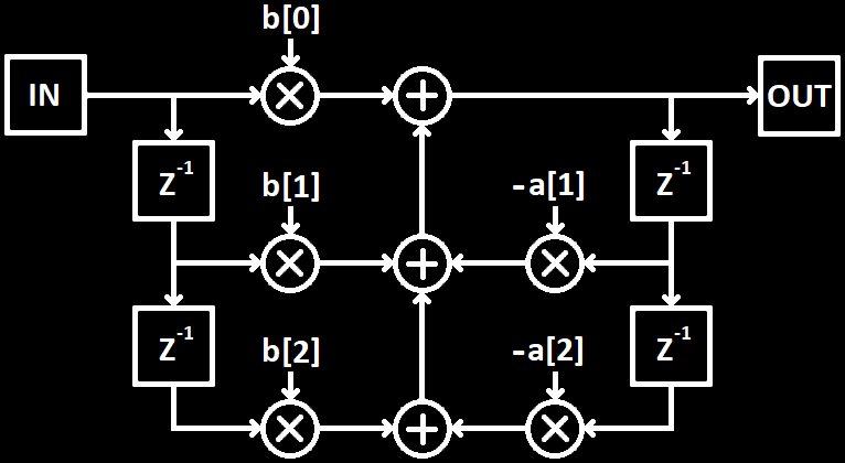
Bellow is a single biquad section, 2nd order IIR filter, where $ Z^{-1} $ is a delay of 1 sample and b[N] are the coefficients for each Tap on the input side (feed-forward) and a[N] are the coefficients for each Tap on the output side (feed-back):

A IIR filter can be designed with SciLab by using the iir(n,ftype,fdesign,frq,delta) function. It uses 5 parameters:

• n: Filter Order
• ftype: Filter type: ‘lp’ for low-pass, ‘hp’ for high-pass, ‘bp’ for band-pass, ‘sb’ for stop-band
• fdesign: The analog filter design used as basis: ‘butt’ for Butterworth, ‘cheb1’ and ‘cheb2’ for Chebyshev, ‘ellip’ for Ellipsis
• frq: Vector of two frequencies for the first and second cut-off frequency (‘lp’ and ‘hp’ only use the first one)
• delta: Vector of two error values for ‘cheb1’, ‘cheb2’ and ‘ellip’ filter.

The function returns the transfer function for the IIR filter.

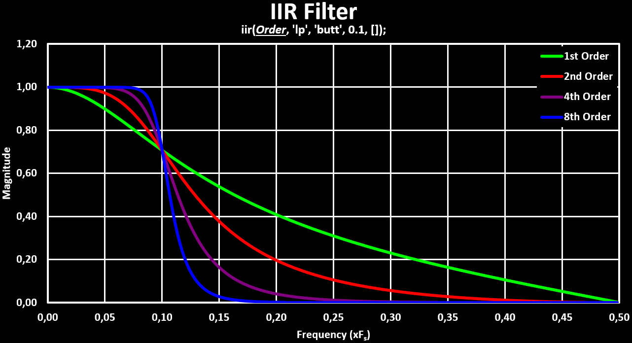
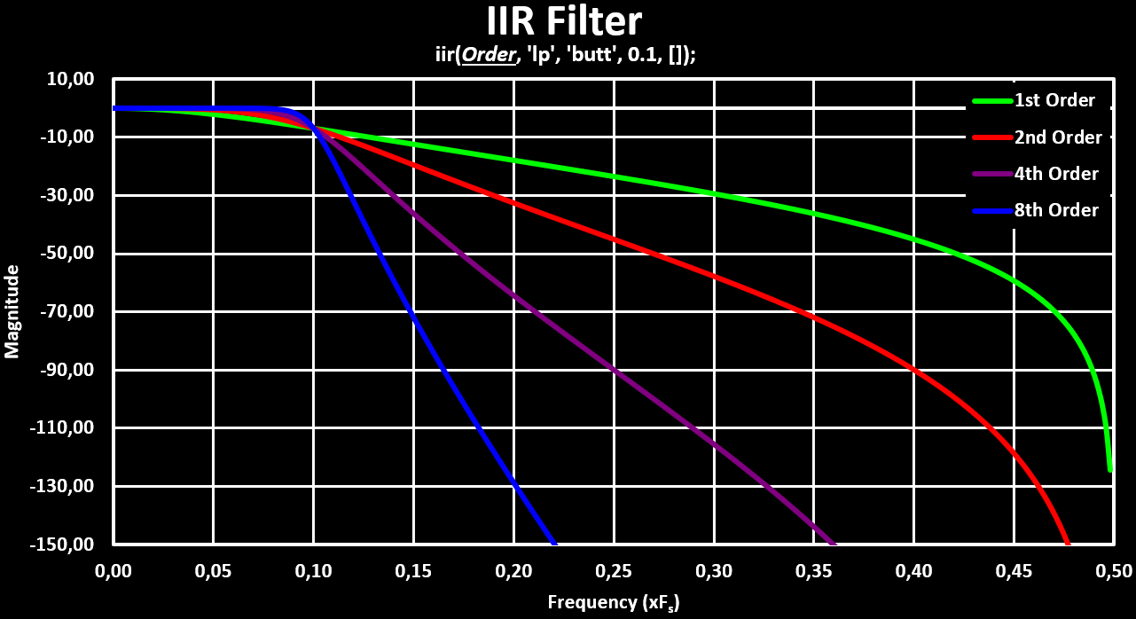
To get/draw the filter response the function frmag(sys,npts) is used where the first parameter, sys, is the transfer function and the second, npts, the number of points to calculate for the frequency response. Bellow is an example of using all these to draw the frequency response of a IIR low-pass filter of order 2 and a cut-off frequency of $ 0.1 * F_{S} $:

hz = iir(4, 'lp', 'butt', 0.1, []);		//Generate IIR Filter Transfer Function
[hzm, fr] = frmag(hz, 256);				//Generate Filter Response Curve
plot(fr', hzm');						//Draw Filter Response Curve

Bellow is a figure that shows the change of the frequency responses with the increase of the filter order. Both in linear magnitude and in logarithmic magnitude, $ 20 * log(mag) $, form:

Linear Log (dB)

To get the actual coefficients of the IIR filter, the transfer function returned by iir(n,ftype,fdesign,frq,delta) has to be evaluated for the delay operator, $ z^-1 $. This can be done by the following SciLab code:

hz = iir(4, 'lp', 'butt', 0.1, []);		//Generate IIR Filter Transfer Function
q = poly(0, 'q');						//To express the result in terms of the delay operator q=z^-1
hzd = horner(hz, 1/q);					//Evaluates the polynomial by substituting the variable z in hz by 1/q

coeffsA = coeff(hzd.den);				//Get a[N] feed-back coefficients
coeffsB = coeff(hzd.num);				//Get b[N] feed-forward coefficients

This gives the IIR feed-back (a[N]) and feed-forward (b[N]) coefficients for the Direct Form 1, in the extended unfolded form. Because many implementations of the IIR filter, e.g. the CMSIS-DSP library, use the cascaded biquad form, the transfer function has to first be converted/unfolded into the cascaded biquad form. This is, to factorize the obtained transfer function into 2nd order sections, 2nd order polynomials.

This can be done with the factors(rat) function in Scilab. The function takes the polynomial as input and returns a list of polynomials of order 1 or 2 for both the numerator (lnum) and denominator (lden) as well as the “gain” (g). With this the biquad sections can now be designed by paring numerator and denominator polynomials, distributing the gain and to normalize the sections so that the denominators are in the form $ ax^2 + bx + 1 $

[lnum, lden, g] = factors(hzd,'d');

Implementation on ARM MCU (CMSIS-DSP)

The CMSIS-DSP library provides functions for the implementation of the Biquad Cascade Direct Form 1 IIR filter in fixed point format, both Q15 and Q31, as well as in float format in F32 (because of the error accumulation problems in the Direct Form 2, the library only provides functions for floats and doubles). A good resource to see how to use each function can be found on this page.

The first thing to do is to initialize the filter structure by using the arm_biquad_cascade_df1_init_q15(S, numStages, pCoeffs, pState, postShift) or arm_biquad_cascade_df1_init_q31(S, numStages, pCoeffs, pState, postShift) or arm_biquad_cascade_df1_init_f32(S, numStages, pCoeffs, pState) functions. These functions expect 5, 4 in case of float, parameters:

• S: Pointer to the filter structure (arm_biquad_casd_df1_inst_q15, arm_biquad_casd_df1_inst_q31, arm_biquad_casd_df1_inst_f32)
• numStages: Number of Taps of Cascaded Biquad Stages
• pCoeffs: Pointer to the filter coefficient array
• pState: Pointer to a state buffer array (used internally as the delay line under others)
• postShift: Shift to be applied to the accumulated result for when the coefficients are not in the Q15/Q31 format

After that, for the fixed-point version, the coefficients have to be convert into the appropriate fixed point format. For Q15 this is done by multiplying the coefficients by $ 2^{15} $ and for Q31 by $ 2^{31} $, and then rounding them to an integer. In case at least one coefficients is over 1, don’t fit in the Q15/Q31 format, all coefficients have to be converted into the format where the largest coefficient fit. For example, when a[1] is 1.049 all coefficients have to be converted into Q14/Q30 by multiplying them by $ 2^{14} $ or $ 2^{30} $. For this case the postShift parameter has to be set to 1 to get the correct filter result.

The coefficients have to be arranged in the following order: b[0], b[1], b[2], a[1], a[2] and then again b[0], b[1], b[2], a[1], a[2] for the next stages. In the Q15 case, there is an additional 0 “coefficient” in-between b[0] and b[1] (b[0], 0, b[1], b[2], a[1], a[2]) used for optimized ALU usage internally. Care has to be taken with the sign of the a[n] coefficients, the CMSIS-DSP implementation uses the coefficients directly with there sign in the multiplication, and often design tools expect them to be used with the “-” sign, as is shown in the block diagram. The coefficients calculated with Scilab is one of those cases, which means that the a[n] coefficients have to be negated to be used in the CMSIS-DSP functions. The state buffer has to be of length $ 4*numStages $ for all versions.

Bellow is example code used to initialize each version of the IIR filter, for a 4th Order Low Pass aka two cascaded biquad sections. The coefficient values used are obtained with the above expressions and with a gain splitting of 50/50:

//Q15 IIR Filter
int16_t irrStateQ15[8];
int16_t iirCoeffQ15[12] = {	779, 0, 1557, 779, 17180, -4852,		//Stage 1: b[0], 0, b[1], b[2], a[1], a[2]
							1663, 0, 3326, 1663, 21642, -10367 };	//Stage 2: b[0], 0, b[1], b[2], a[1], a[2]
arm_biquad_casd_df1_inst_q15 armIIRInstanceQ15;
arm_biquad_cascade_df1_init_q15(&armIIRInstanceQ15, 2, iirCoeffQ15, irrStateQ15, 1);

//Q31 IIR Filter
int32_t irrStateQ31[8];
int32_t iirCoeffQ31[10] = {	51021742, 102043591, 51021742, 1125925247, -317978333,		//Stage 1: b[0], b[1], b[2], a[1], a[2]
							109014001, 218028109, 109014001, 1418319963, -679398113 };	//Stage 2: b[0], b[1], b[2], a[1], a[2]
arm_biquad_casd_df1_inst_q31 armIIRInstanceQ31;
arm_biquad_cascade_df1_init_q31(&armIIRInstanceQ31, 2, iirCoeffQ31, irrStateQ31, 1);

//Float IIR Filter
float irrStateF32[8];
float iirCoeffF32[10] = {	0.0475f, 0.095f, 0.0475f, 1.049f, -0.296f,	//Stage 1: b[0], b[1], b[2], a[1], a[2]
							0.1015f, 0.203f, 0.1015f, 1.321f, -0.633f };	//Stage 2: b[0], b[1], b[2], a[1], a[2]
arm_biquad_casd_df1_inst_f32 armIIRInstanceF32;
arm_biquad_cascade_df1_init_f32(&armIIRInstanceF32, 2, iirCoeffF32, irrStateF32);

After the initialization the filter is now ready to be used. To apply the filter to a new input sample the arm_biquad_cascade_df1_q15(S, pSrc, pDst, blockSize) or arm_biquad_cascade_df1_q31(S, pSrc, pDst, blockSize) or arm_biquad_cascade_df1_f32(S, pSrc, pDst, blockSize) function is called, which expects 4 parameters:

• S: Pointer to the filter structure
• pSrc: Pointer to the input samples (an array when block size > 1)
• pDst: Pointer to where write the output filtered samples (an array when block size > 1)
• blockSize: Block length, how many samples to process in one call

Bellow is example code on how to use each of these filter functions. In case of the fixed point implementations, there is a _fast version for each of them that is slightly faster but does not do any overflow protection and so the input has to be scaled to prevent overflow, by 2 bits into the [-0.25; 0.25] range. In general, the performance gain is so minimal that it is not worth the complications that can happen, as can be seen in the benchmark section.

//Q15 FIR Filter
uint32_t blockLen = 1;
int16_t inputSample;
int16_t filteredSample;
arm_biquad_cascade_df1_q15(&armIIRInstanceQ15, &inputSample, &filteredSample, blockLen);
//Slightly faster but no overflow protection
//arm_biquad_cascade_df1_fast_q15(&armIIRInstanceQ15, &inputSample, &filteredSample, blockLen);

//Q31 FIR Filter
uint32_t blockLen = 1;
int32_t inputSample;
int32_t filteredSample;
arm_biquad_cascade_df1_q31(&armIIRInstanceQ31, &inputSample, &filteredSample, blockLen);
//Slightly faster but no overflow protection
//arm_biquad_cascade_df1_fast_q31(&armIIRInstanceQ31, &inputSample, &filteredSample, blockLen);

//Float FIR Filter
uint32_t blockLen = 1;
float inputSample;
float filteredSample;
arm_biquad_cascade_df1_f32(&armIIRInstanceF32, &inputSample, &filteredSample, blockLen);

Cascaded Integrator-Comb (CIC) filter is an optimized version of the moving average FIR filter. It is based on the recursive implementation of it where instead of summing N samples together the newest sample ($ x[n] $) is added to the previous output ($ y[n - 1] $) and the oldest sample ($ x[n - M] $) is subtracted. This is, with the gain scaling factor omitted (division by M):

$$ y[n] = \sum_{k=0}^{M-1} x[n - k] = y[n - 1] + x[n] - x[n - M] $$

The CIC filter implements this with two sections: the comb section which implements the delayed subtraction ($ c[n] = x[n] - x[n - M] $), and the integrator section which implements the feedback part ($ y[n] = y[n - 1] + c[n] $). The basic CIC filter is a integrator section followed by a comb section where the delay line length (M) of the comb section defines the cut-off frequency, equivalent to the number of samples summed in the moving average filter. The block diagram for the basic CIC filter can be seen in the figure bellow:

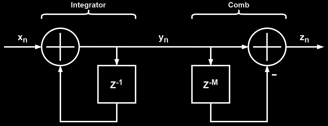
Rewriting the above block diagram by using the z-transform transfer functions for the comb and integrator section gives the following block diagram, with the corresponding time-domain difference equation for each block written bellow them:

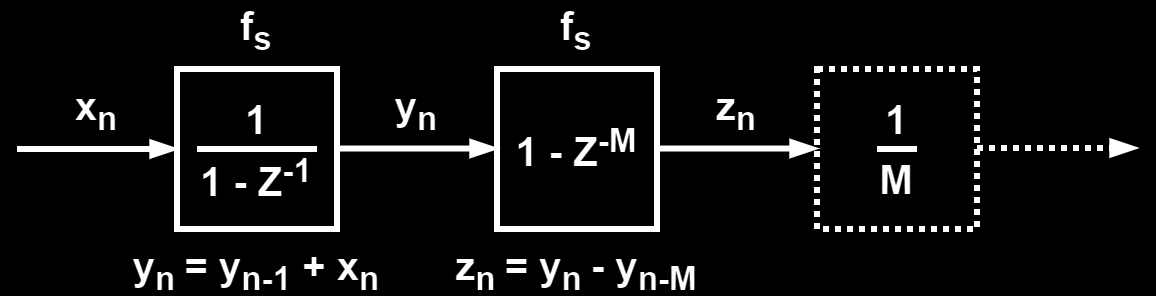
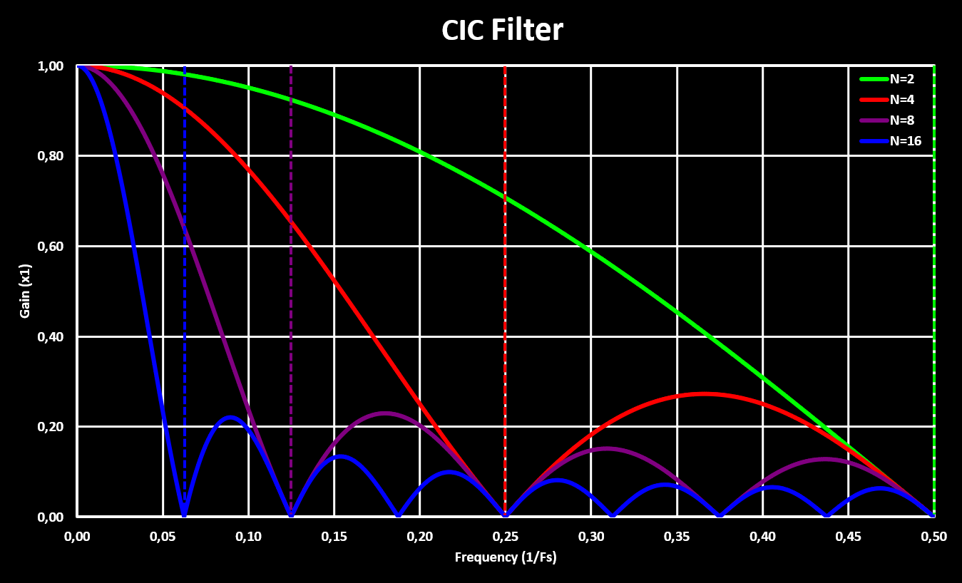
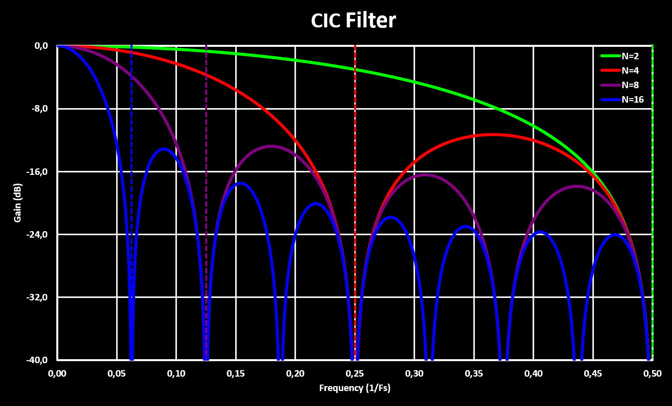
The basic CIC filter, with the architecture shown in the block diagrams above, has the same frequency response as a moving average filter and is given by the equation bellow:

$$ H({f \over f_s}) = \left | {{1 \over M} {{\sin (2 \pi f {M \over 2})} \over {\sin (2 \pi {f \over 2})} }} \right | $$

This gives a response shown in the figures bellow, for different delay line lengths and in both linear and logarithmic gain scale.

Linear Log (dB)

Higher orders CIC filters are achieved by cascading multiple CIC filters, with the comb and integrator sections rearranged so that they are grouped together. This is possible because both the comb and integrator sections are linear time-invariant (LTI) systems which allows the rearranging without modifying the result. It is important to note that with multiple stages the gain scaling factor gets very large quick as now it not only depends on the number of samples in the delay line (M) but also on the number of stages (S), and exponentially with those! A simple multi-stage CIC filter is shown in the block diagram bellow:

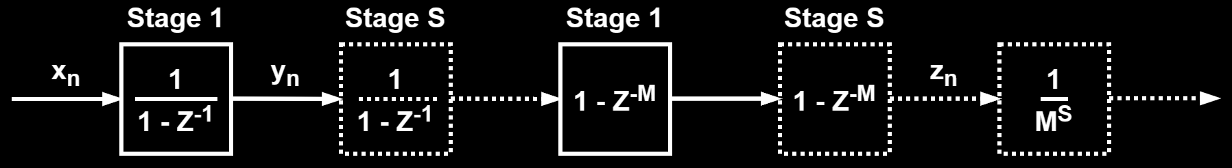
The figures bellow show the frequency response of a 8 samples CIC filter with different number of stages:

Linear Log (dB)

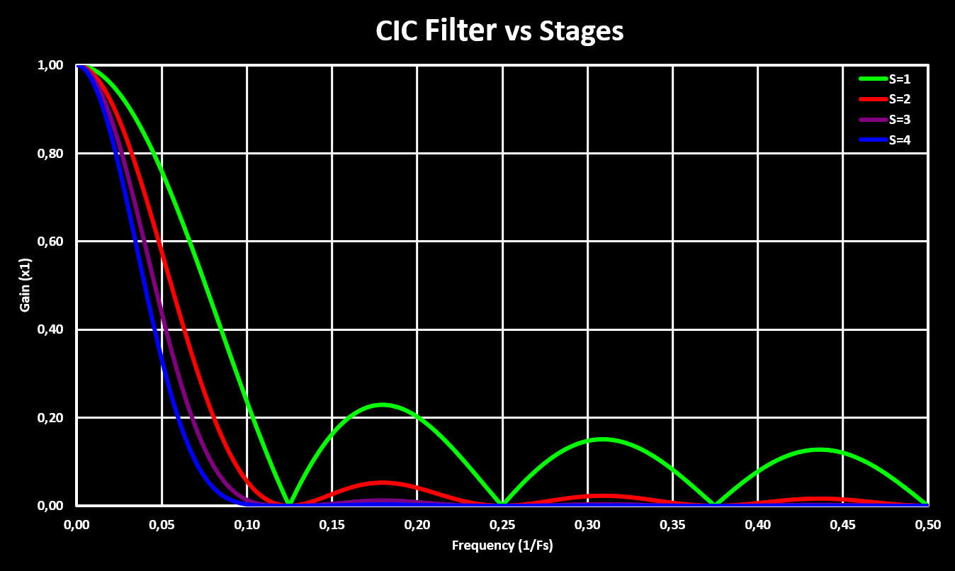
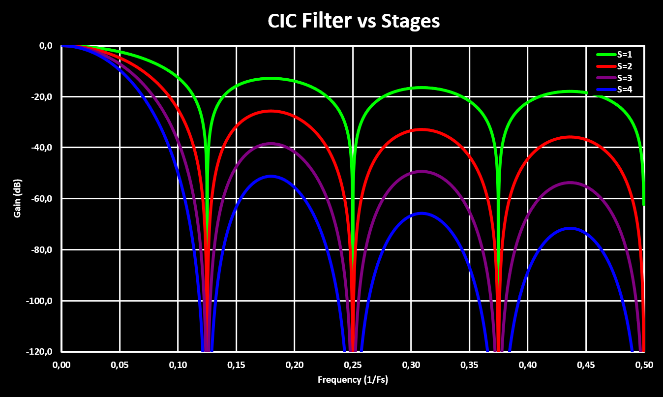
An important note is that, in contrast to other digital filter like FIR or IIR, the CIC filter can only be implemented with fixed-point notation (no floats!) because it relays on the overflow characteristics of fixed-point math. Also, a great article on CIC filters and simple compensation with some more in-depth explanations can be found here.

CIC Decimator

CIC filters are specially interesting when used in combination with decimation (or interpolation). Because the decimation operation is also a LTI operation, it can be moved into the CIC filter and fitted between the integrator and comb sections. With this arrangement, the size of the delay line of the comb section is reduced by the decimation ratio. On the limit, when the decimation ratio is the same as the comb section delay line length (M), to only one sample. The block diagram for a CIC decimator with the same decimation ratio as the original CIC filter delay line length is shown in the figure bellow:

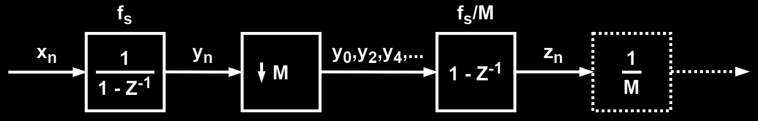
This represents the most commonly used implementation, the CIC filter bandwidth and the decimation ratio coincide and the resulting decimation filter is extremely simple. It only uses two sums, no multiplications, and when the decimation factor is a power of 2 the gain scaling can be achieved with a simple right shift. This makes the CIC decimation architecture the preferred choice for systems that require decimation, specially in FPGAs and integrated circuits e.g. in high resolution ADCs or compact digital transceivers.

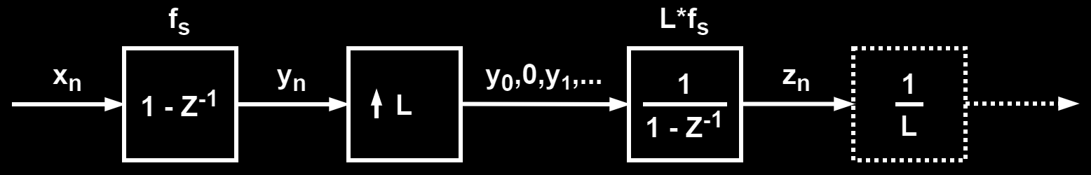
CIC Interpolator

Another popular application for CIC filters is in interpolation. As with decimation, the interpolation stage is also integrated into the CIC filter but with the order of the comb and integrator stages swapped. Again this is made possible because of the LTI nature of interpolation. By arranging the sections in this way the delay line can be reduced by the interpolation ratio. On the limit, when the interpolation ratio is the same as the comb section delay line length (M), to only one sample. The interpolation stage performs zero-stuffing, adding L zeros between two consecutive samples. The block diagram for a CIC interpolator with the same interpolation ratio as the original CIC filter delay line length is shown in the figure bellow:

Compensation Filter

Because CIC filters don’t have a very flat frequency response in the pass-band they are often followed by a compensation filter. This compensation filter is normally implemented as a FIR filter and is designed to have a frequency response with the inverse characteristics of the CIC filter, flattening the overall response. This makes for a great overall decimation, or interpolation, filter and because the compensation filter is put either after the decimation or before the interpolation it always runs on the lower sampling rate, making it still more efficient then doing the decimation/interpolation with a FIR filter directly.

There are many different techniques to design the FIR compensation filter, with the easiest and most straight forward being using frequency sampling. Using frequency sampling allows to design the compensation FIR filter by sampling the exact response that is desired, normally the inverse of the CIC filter with a low-pass “window” added to improve the attenuation outside the required bandwidth. In Matlab this can be done with the fir2 function, the approach used in a application note from Intel/Altera: Understanding CIC Compensation Filters. But there is no equivalent in Scilab, no frequency response sampling method that returns the FIR filter coefficients…

To overcome this, a custom frequency sampling function was implemented (good article about frequency sampling can be found here), as well as a function that returns the inverse CIC response and low-pass “window” function. A wrapper function, CICCompFilter(m,d,fc,bp,n), is also implemented so that the compensation filter can easily be adjusted to fit the application by setting the following 5 parameters:

• m: CIC filter delay line length
• d: Decimation ratio
• fc: Low-pass cut-off frequency
• bp: Low-pass transition bandwidth
• n: Number of Taps (should be odd)

The function returns the FIR filter coefficients, the sampled points and a RMS value of the error to the ideal filter. The filter design is also drawn in a graph with plots showing the design parameters. The source code file can be downloaded from the link bellow:

Scilab code file: CICCompFilter.sce

As an example, a compensation filter for a CIC with a delay line length of 8, decimation factor of 8, a cutoff frequency of 0.25 and a transition band of 0.1 with 11 taps is designed:

hn = CICCompFilter(8, 8, 0.25, 0.1, 11);	//Generate FIR Filter Coefficients

The figure bellow shows the obtained filter response (red) together with the CIC filter (purple) response and inverse of it (purple dashed), the low-pass “window” (white dashed), the ideal/desired filter response (green) and the global response (blue) of the CIC followed by the compensation filter:

Linear Log (dB)

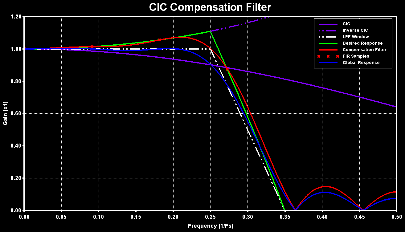
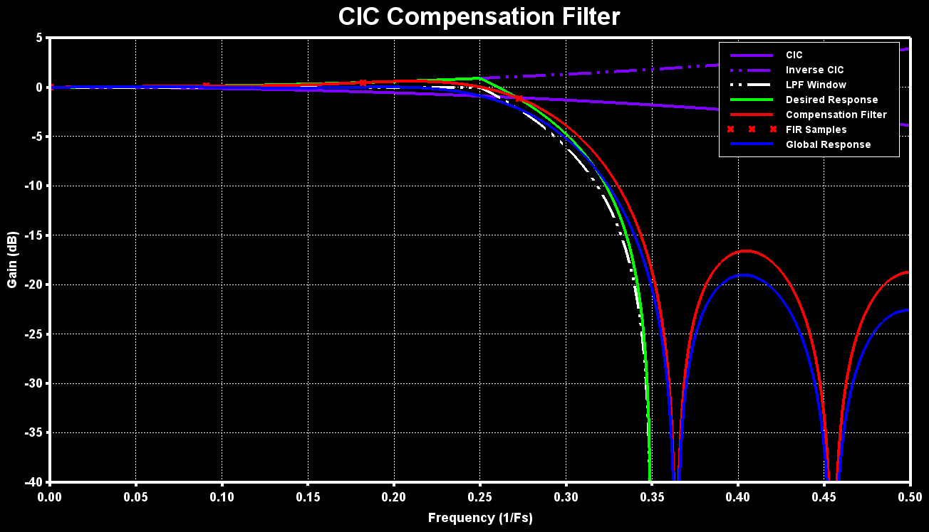
Implementation on ARM MCU

The CMSIS-DSP library doesn’t provide functions for any CIC filters so a costume implementation has to be realized. Bellow is a working implementation for all three CIC filters: the basic filter, the decimation filter and the interpolation filter. The API is based on the CMSIS-DSP library API and should be easy to understand and use. These implementations are not highly optimized but they work and serve as a basis and example for a implementation in C for embedded systems.

Source file: dspCICFilter.c

Header file: dspCICFilter.h

(NOTE: Currently only the decimation filter supports multiple stages)

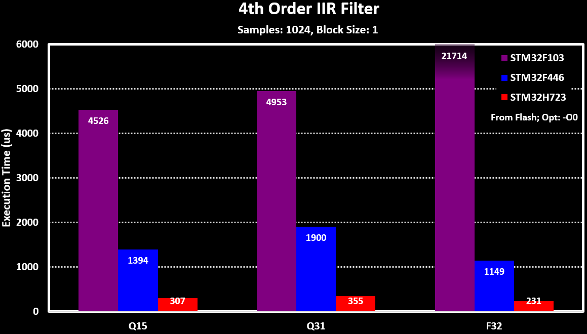
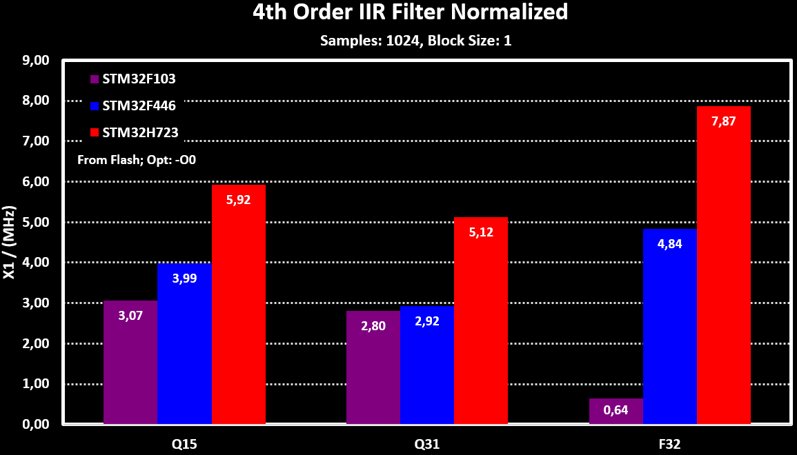
The ARM CMSIS-DSP library filters were tested on different MCUs, with different ARM Cortex-M cores, to evaluate there performance. The base test is running the filter over a 1024 samples sized array and measure the time it takes to complete. This is then repeated 10 times and average is calculated.

The MCUs tested are:

• STM32F103: An ARM Cortex-M3 with no FPU and no cache, 20 kB RAM and clocked at 72MHz
• STM32F446: An ARM Cortex-M4f with FPU and no cache, 128 kB RAM and clocked at 180MHz
• STM32H723: An ARM Cortex-M7 with FPU and 32/32 kB D-/I-Cache, 564 kB RAM and clocked at 550MHz

Bellow are the results for the different MCUs, both in $ \mu s $ and normalized for the clock frequency (x1/MHz):

Time Normalized (1/MHz)

More detailed tests

With the STM32H723, more detailed performance tests where realized:

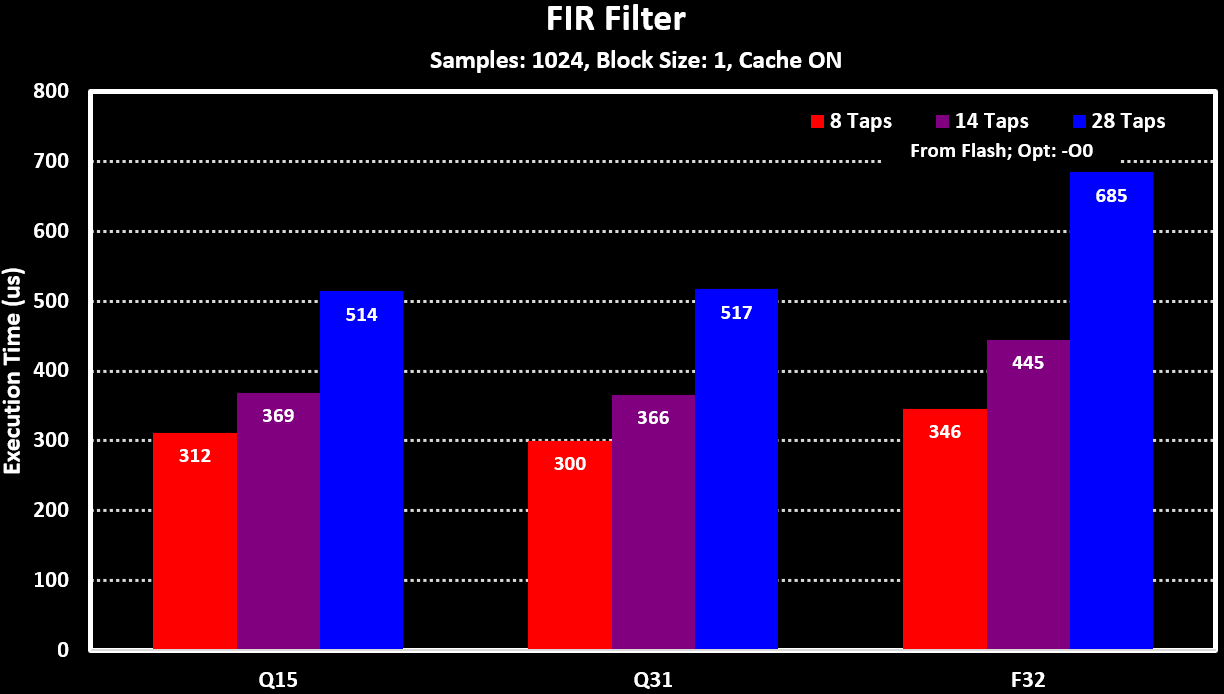
With different Taps counts for FIR filter:

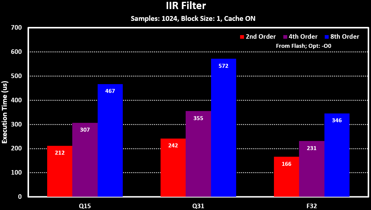
With different filter orders for the IIR filter, number of biquad sections:

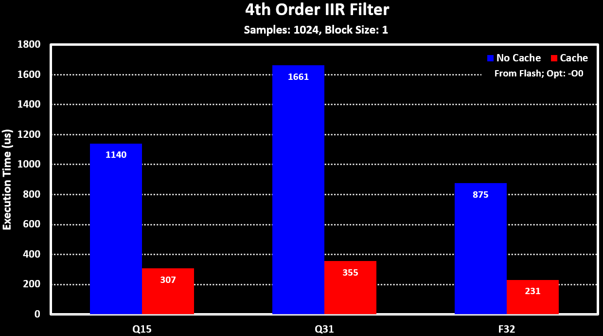
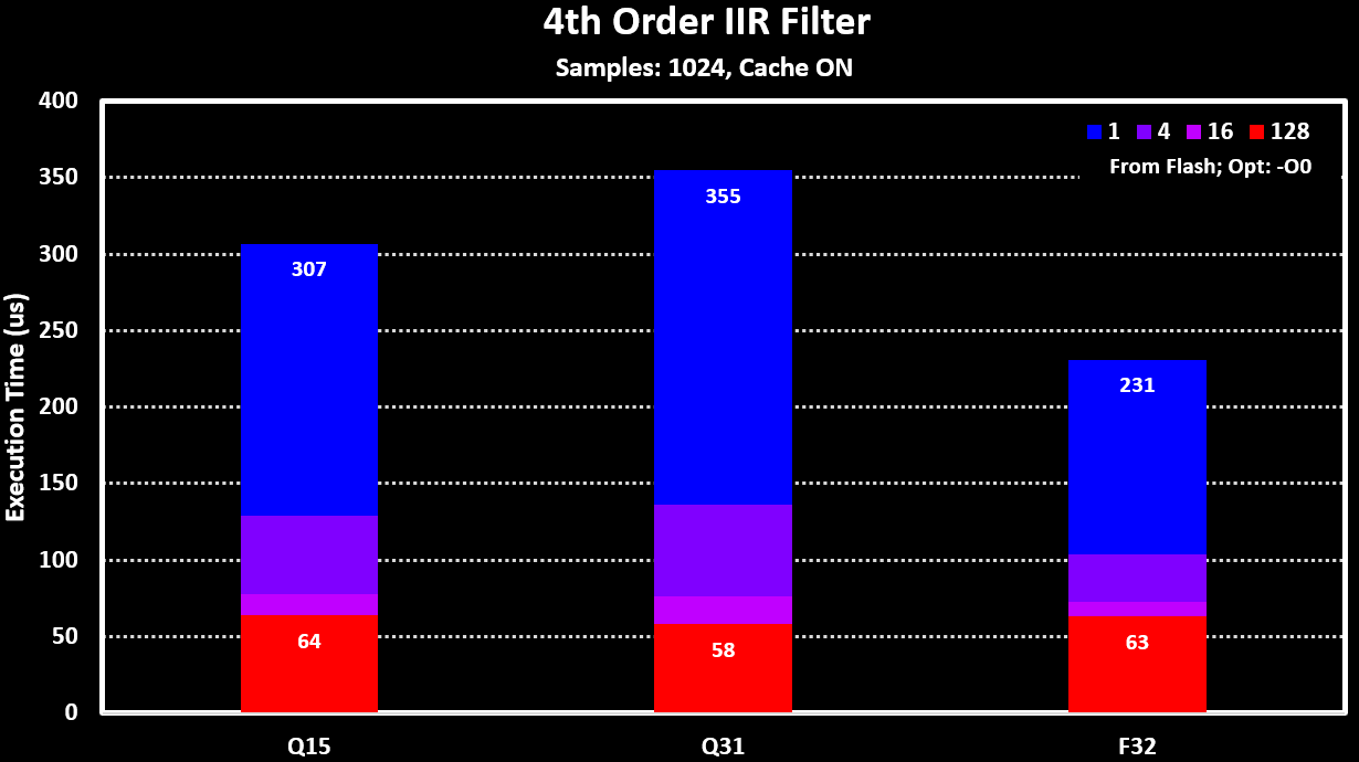
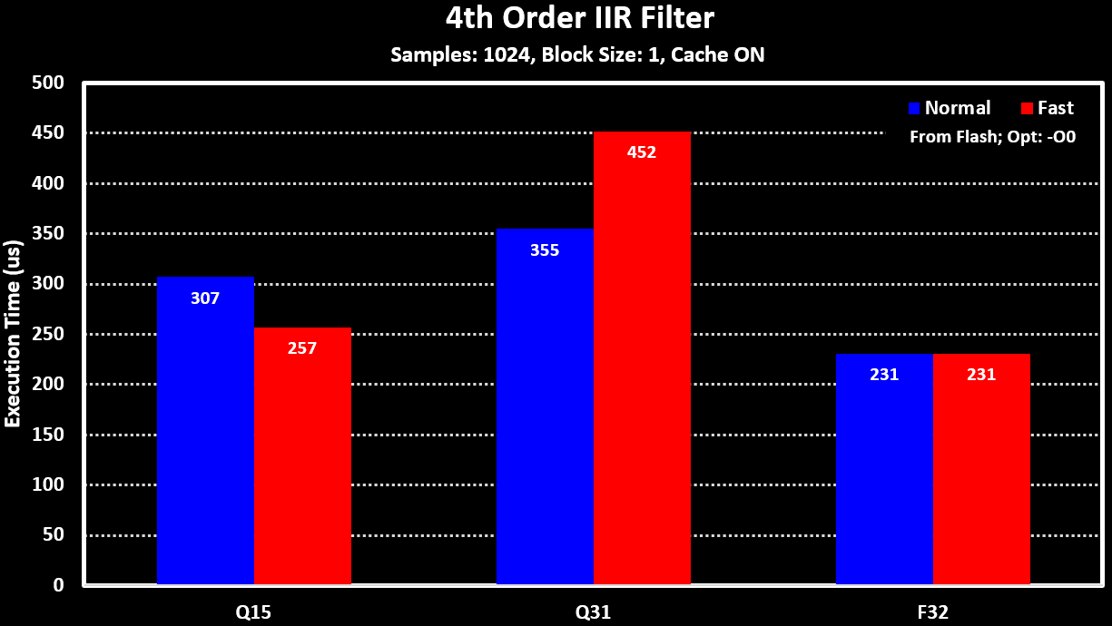
To see the impact of the processing block size and the _fast filter functions for the fixed-point versions (“xx_fast_q15” and “xx_fast_q31”), the 4th Order IIR Filter is used. The results for these can be seen in the figure bellow:

Block Size Normal vs Fast

As the STM32H723 has large cache of 32 KB of both I and D cache, the performance impact of using or not the cache was also tested and can be seen in the figure bellow: